Mastering Excel: How to Easily Make All Cells the Same Size in Excel
Excel is an incredibly powerful tool that can help you organize, analyze, and visualize data. However, if you’re not careful, it can also be a bit overwhelming. One of the most common challenges people face when working with it is how to make all cells the same size in Excel. Whether you’re trying to make all columns the same size or all rows the same size, it can be a frustrating and time-consuming process.
Fortunately, there are several easy ways to make all cells the same size in Excel. One popular method is to use the “AutoFit” feature, which automatically adjusts the width of columns and the height of rows to fit the contents of the cells. Another option is to manually adjust the column width or row height by selecting the cells you want to adjust and dragging the boundary of one of the selected cells to the desired size.
Whether you’re a seasoned Excel pro or a beginner just starting out, learning how to make all cells the same size can save you time and frustration in the long run. By following a few simple steps, you can ensure that your data is organized, easy to read, and visually appealing. So why wait? Start exploring the many ways to make all cells, columns, and rows the same size in Excel today!
Adjusting Column Width and Row Height
Excel allows you to adjust the width of columns and height of rows to make all cells the same size. Here’s how you can do it:
Adjusting Column Width
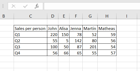
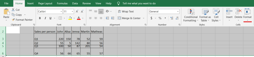
To adjust the width of all columns in Excel, you can use the AutoFit Column Width feature. This will automatically adjust the width of all columns to fit the content within them. To use this feature, select all the columns you want to adjust, then click on the Home tab and select Format in the Cells section.

From the drop-down menu, select AutoFit Column Width.

For our example, it looks like this:
If you want to adjust the width of all columns to a specific size, you can use the Column Width feature. To do this, select all the columns you want to adjust, then click on the Home tab and select Format in the Cells section.
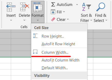
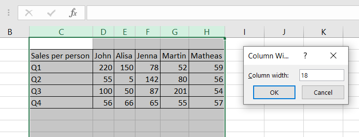
From the drop-down menu, select Column Width. In the Column Width dialog box, enter the desired width and click OK.
Adjusting Row Height
To adjust the height of all rows in Excel, you can use the AutoFit Row Height feature. This will automatically adjust the height of all rows to fit the content within them. To use this feature, select all the rows you want to adjust, then click on the Home tab and select Format in the Cells section.
From the drop-down menu, select AutoFit Row Height.
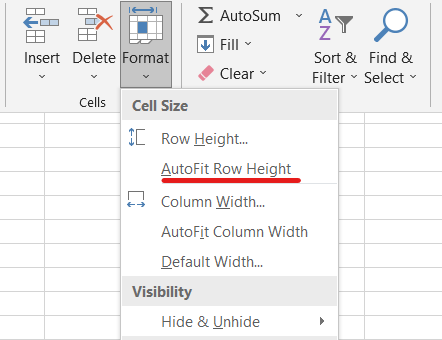
In our case, it turned out like this:
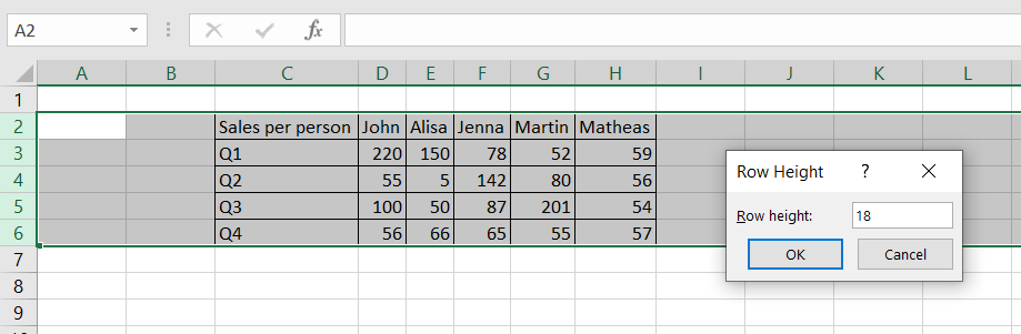
If you want to adjust the height of all rows to a specific size, you can use the Row Height feature. To do this, select all the rows you want to adjust, then click on the Home tab and select Format in the Cells section. From the drop-down menu, select Row Height.
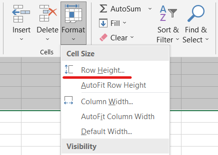
In the Row Height dialog box, enter the desired height and click OK.
By adjusting the column width and row height, you can make all cells in Excel the same size. Whether you want to adjust all columns to the same size, all rows to the same size, or both, Excel provides several options to help you achieve this.
Thank you for reading this section on adjusting column width and row height in Excel. We hope you found it helpful in making all cells the same size. Stay tuned for more tips and tricks on using Excel!
How to Make All Cells the Same Size in Excel
Making all cells the same size in Excel can make your spreadsheet look more organized and professional. Whether you want to adjust the width of all columns or the height of all rows, Excel offers several simple methods to achieve this. To make all columns the same size, select the column headers of all the cells you want to adjust.
Drag the boundary of any one of the selected column headers to the width you like. When you release the mouse button, you will find all the other selected columns resized to the same width.
Alternatively, you can use the Format option on the Home tab to set the width of all columns to a specific measurement in points, which we covered earlier.
To make all rows the same size, select the row headers of all the cells you want to adjust. Drag the boundary of any one of the selected row headers to the height you like. When you release the mouse button, you will find all the other selected rows resized to the same height.

You can also use the Format option on the Home tab to set the height of all rows to a specific measurement in points as explained previously. If you want to make both columns and rows the same size, select all the cells in the spreadsheet by clicking the triangle in the top left corner of the sheet.
Then, use the same methods described above to adjust the width and height of the cells. In conclusion, making all cells the same size in Excel is a simple process that can make your spreadsheet look more professional and organized. Whether you want to adjust the width of all columns, the height of all rows, or both, Excel offers several methods to achieve this. By following the steps outlined above, you can easily make all cells the same size in your Excel spreadsheet. Thank you for reading!
How to Make All Rows the Same Height in Excel
Excel is an excellent tool for organizing and analyzing data. However, when working with large data sets, it can be challenging to keep your spreadsheet looking neat and organized. One way to improve the appearance of your Excel worksheet is to ensure that all rows have the same height. There are several ways to make all rows in Excel the same height. One way is to use the Row Height command. Here’s how to do it: 1. Select the rows that you want to adjust. You can select a single row or multiple rows by clicking and dragging the mouse pointer over the row headers. 2. Right-click on the selected rows and choose “Row Height” from the context menu. 3. In the “Row Height” dialog box, enter the desired height in the “Row Height” field. 4. Click “OK” to apply the changes. Another way to make all rows the same height is to use the Format Painter tool. Here’s how to do it: 1. Select a row that has the desired height. 2. Click the “Format Painter” button on the “Home” tab. 3. Select the rows that you want to adjust. 4. The selected rows will now have the same height as the original row. If you want to make all rows and columns the same size, you can use the “Select All” command to select the entire worksheet. Then, use the “Row Height” and “Column Width” commands to set the desired size for all rows and columns. In conclusion, making all rows the same height in Excel is a simple process that can help improve the appearance of your worksheet. Whether you use the Row Height command, the Format Painter tool, or the Select All command, you can easily adjust the height of your rows to create a more organized and professional-looking spreadsheet.
How to Make All Columns the Same Width in Excel
Having columns of different widths can make your Excel sheet look messy and unprofessional. Luckily, it’s easy to make all columns the same width in Excel. Here’s how:
First, select the columns you want to adjust. You can do this by clicking and dragging across the column headings, which are the letters at the top of each column. Alternatively, you can click on a single column heading to select just that column.
Once you’ve selected the columns, you can adjust their width by clicking and dragging on the boundary between two column headings. The cursor will change to a double-headed arrow, indicating that you can adjust the width. Drag the boundary to the desired width and release the mouse button. All the selected columns will now be the same width.
If you want to make all columns the same width in the entire sheet, you can select all columns by clicking the box above the column headings that has the letter A and the number 1 in it. This will select the entire sheet. Then, adjust the width of any column as described above. All columns in the sheet will now be the same width.
It’s important to note that adjusting the width of a column can cause text in that column to wrap to the next line if it’s too long to fit in the new width. If you want to avoid this, you can use the “AutoFit” feature to automatically adjust the width of a column to fit its contents. To do this, double-click on the boundary between two column headings. The column will be resized to fit its contents.
Now that you know how to make all columns the same width in Excel, you can create a clean and organized sheet that looks professional and is easy to read.
Using the Format Painter
If you have a specific formatting style that you want to apply to multiple cells in Excel, the Format Painter is a great tool to use. It allows you to copy the formatting from one cell or range of cells and apply it to another cell or range of cells with just a few clicks.
To use the Format Painter, first, select the cell or range of cells that contain the formatting that you want to copy. Then, click on the Format Painter button in the Clipboard group on the Home tab. The cursor will change to a paintbrush icon, indicating that the Format Painter is active.
Next, click on the cell or range of cells where you want to apply the formatting. Excel will automatically apply the formatting to the new cells, making them look exactly like the original cells.
Using the Format Painter can save you a lot of time if you need to apply the same formatting to multiple cells or ranges of cells in your worksheet. It’s a quick and easy way to make your worksheet look more professional and consistent.
However, keep in mind that the Format Painter only copies the formatting, not the content of the cells. So if you need to copy both the formatting and the content of a cell, you’ll need to use a different method, such as copying and pasting the cell.
In summary, the Format Painter is a handy tool in Excel that can help you quickly apply formatting to multiple cells or ranges of cells. It’s easy to use and can save you a lot of time when formatting your worksheet.
Using the Table Feature
If you’re working with a lot of data, using the table feature in Excel can be a lifesaver. It makes it easy to sort, filter, and format your data. Plus, tables have built-in functionality that makes it simple to make all the cells the same size.
To create a table, select your data and then click the “Insert” tab. From there, click “Table.” Excel will automatically detect the range of cells you’ve selected, and you can choose whether or not to include headers. Once you’ve created your table, you can start formatting it.
If you want to make all the columns the same size, simply click on a column header to select the entire column. Then, drag the boundary of the column to the width you want. Excel will automatically adjust all the other columns to the same width.
To make all the rows the same size, click on a row header to select the entire row. Then, drag the boundary of the row to the height you want. Excel will automatically adjust all the other rows to the same height.
Using the table feature in Excel is a great way to keep your data organized and easy to read. By making all the cells, columns, and rows the same size, you can create a polished and professional-looking spreadsheet in no time.
Now that you know how to use the table feature to make all the cells the same size in Excel, you’re well on your way to becoming an Excel pro. Keep practicing and exploring all the features Excel has to offer, and you’ll be a master in no time!
Using the Alignment Tools
Excel provides several alignment tools to help users align text and data in cells. These tools can also be used to make all cells the same size. To change text alignment in Excel, select the cell(s) you want to realign, go to the Home tab > Alignment group, and choose the desired option.
If you want to align data vertically, click one of the following icons: Top Align – aligns the contents to the top of the cell. Middle Align – aligns the contents to the middle of the cell. Bottom Align – aligns the contents to the bottom of the cell. You can also choose to justify the text in a cell. Justifying the text will align the text to both the left and right margins of the cell.
To make all columns the same size, select the column headers of all the cells you want to adjust. Drag the boundary of any one of the selected column headers to the width you like. When you release the mouse button, you will find all the other selected columns resized to the same width.
To make all rows the same size, select the row(s) of interest, go to the Home tab > Cells group, and click Format > AutoFit Row Height. This will adjust the height of all selected rows to match the size of the largest cell in the row.
Using the alignment tools in Excel can help you make all cells the same size quickly and easily. Whether you need to adjust the width of columns or the height of rows, these tools will make the process simple and straightforward.
Remember, keeping your Excel spreadsheets organized and consistent is key to making sure they are easy to read and understand. By using the alignment tools and other formatting options available in Excel, you can create professional-looking spreadsheets that are both functional and aesthetically pleasing.
Using the Autofit Feature
One of the easiest ways to make all cells the same size in Excel is by using the Autofit feature. This feature allows you to adjust the width and height of your cells to match the size of your data. Here’s how to use the Autofit feature to make all columns and rows the same size:
Autofit Columns
To Autofit columns, select one, several or all columns on the sheet, go to the Home tab > Cells group, and click Format > AutoFit Column Width. This will adjust the width of the columns to match the size of your data. You can also use the keyboard shortcut Ctrl+Shift+F to Autofit columns.
Autofit Rows
To Autofit rows, select the row(s) of interest, go to the Home tab > Cells group, and click Format > AutoFit Row Height. This will adjust the height of the rows to match the size of your data. You can also use the keyboard shortcut Ctrl+Shift+F to Autofit rows.
Autofit All Cells
If you want to Autofit both columns and rows, you can combine the two commands using a macro. Here’s how:
| Step | Action |
|---|---|
| 1 | Open your spreadsheet in Microsoft Excel. |
| 2 | Click the worksheet in which you want to use AutoFit. |
| 3 | Select the entire worksheet by clicking the “Select All” icon (a diagonally-pointed triangle) in the worksheet’s top-left corner. |
| 4 | Press Alt+F11 to open the Visual Basic Editor. |
| 5 | Click Insert > Module to create a new module. |
| 6 | Paste the following code: Sub autofitAllCells () Selection.Columns.AutoFit Selection.Rows.AutoFit End Sub |
| 7 | Press F5 to run the macro. |
| 8 | Close the Visual Basic Editor and return to your worksheet. |
By following these steps, you can easily make all cells the same size in Excel using the Autofit feature. Whether you want to adjust the width of your columns or the height of your rows, Autofit makes it easy to ensure that your data is presented in a clear and organized way.
Thank you for reading, and happy Excel-ing!
Using the Keyboard Shortcut
Another quick and easy way to make all cells the same size is by using a keyboard shortcut. This method is perfect for those who prefer using their keyboard over a mouse.
To make all cells in a row or column the same size, simply select the row or column you want to adjust. Then, hold down the “Ctrl” key on your keyboard and press the “Shift” key. Finally, press the “0” key. This will adjust the size of the selected rows or columns to match the size of the largest row or column in the selection.
If you want to make all cells in the entire worksheet the same size, simply press “Ctrl + A” to select all cells, and then use the same keyboard shortcut as before.
It’s important to note that this method will adjust the size of all cells in the selected rows or columns, regardless of whether there is any content in them. If you only want to adjust the size of cells that contain content, you can use the “AutoFit” feature instead.
Overall, using the keyboard shortcut is a quick and efficient way to make all cells the same size in Excel. Whether you want to adjust the size of a single row or column, or the entire worksheet, this method can help you get the job done in no time.
Conclusion
Now that you know how to make all cells the same size in Excel, you can easily format your spreadsheets to look more professional and organized. Whether you want to make all columns the same size or all rows the same size, there are several methods you can use to achieve your desired result.
Using the column width command is a quick and easy way to make all columns the same size. Simply select the column headers of all the cells you want to adjust and drag the boundary of any one of the selected column headers to the width you like. When you release the mouse button, all the other selected columns will be resized to the same width.
If you prefer to select particular rows and columns to make the cells the same size in Excel, you can do so by highlighting the desired cells and using the mouse to fix the cell size manually. Alternatively, you can choose the AutoFit option to fix column width and row height in Excel.
Finally, if you want to resize all columns and rows to exact sizes, you can use the Format option on the Home tab. In the Cells section of the ribbon, select the Format drop-down arrow and pick either “Column Width” or “Row Height.” Enter the measurement in points for the columns or rows and click “OK.”
By using these methods, you can easily make all cells the same size in Excel and present your data in a clear and organized manner. Thank you for reading and happy spreadsheet formatting!